
Blog & Design Guide

Motor drive PCB layout must provide a short high-frequency connection between the local DC-link capacitance and the switching power stage. Motor phase current alone does not describe that connection. During a switching transition, current transfers between semiconductor paths while the inductive load current changes much more slowly. The geometry of the commutation connection therefore deserves a separate review from the DC current rating of the power copper.
Begin with the switch states and the actual return connection. Then estimate the voltage contribution from a stated loop inductance and current slope. Finally, examine how much charge the local capacitor must supply before the more distant source responds. The examples below use hypothetical inputs to expose those relationships. They are not component-selection limits, measured inverter results, or manufacturing capability promises.
Follow the switching event
Take one phase leg of an inverter and identify the high-side switch, low-side switch, and their shared phase node. For a selected current direction, draw the conducting path before the switching event and the path after it. Include diode or reverse-channel conduction during the applicable interval. The other phase leg and motor winding complete the load-current path even when a simplified sketch leaves them outside the drawing.
The sections common to both states carry the continuing load current. The sections where current changes quickly form the high-frequency commutation connection. Its inductance includes more than the visible top-layer trace. Capacitor terminations, connecting copper, vias, device leads, and package interconnects all contribute. Decide which of these are included in any quoted inductance before comparing two estimates.
The topology sketch identifies the local capacitor and one half-bridge. The colored arrows indicate connection directions used in explaining commutation, not an instruction to turn both switches on together. The motor and the return phase leg lie outside this simplified drawing.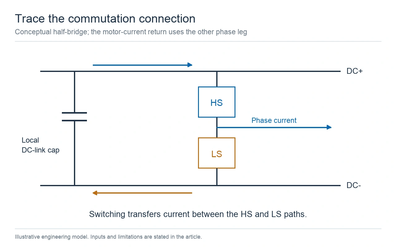
One half-bridge connection is shown; the paths represent different switching states, not simultaneous switch conduction.
The TI motor-driver board-layout application note, revision B separates bulk capacitance, local bypass placement, and power-stage routing. Its examples are useful for identifying the connections that need review. Their package layouts and component recommendations remain specific to the devices and conditions described in the note.
A bulk capacitor near the power entry can supply a slower current transient, yet its route to a phase leg may still be too inductive for the fastest edge. Identify the nearby capacitance connected across the local power-stage supply. Follow both terminals all the way to the semiconductor path. A capacitor positioned beside a switch can have a long connection if its return travels around a slot or through a narrow neck.
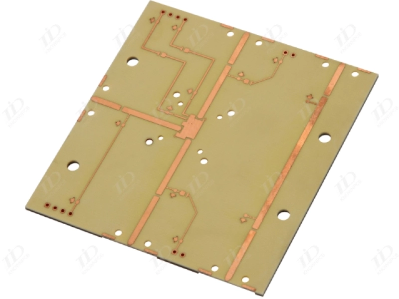
The board photograph shows broad copper areas and local routing features on an unassembled PCB. It provides physical context for a power-copper discussion. It is not identified here as the motor-drive circuit used in the calculations, and no loop inductance can be read from its photograph.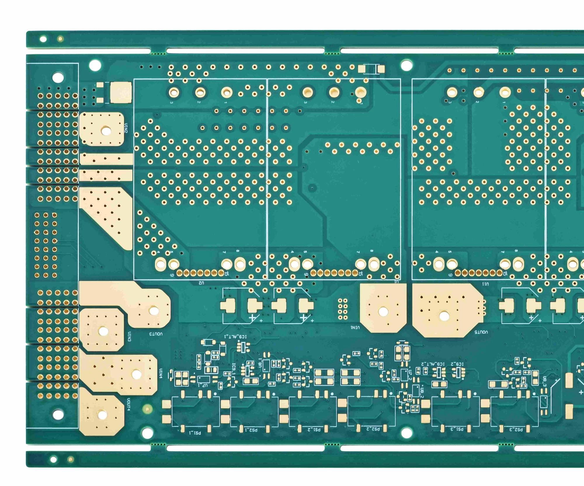
General bare-board copper geometry; this is not a measured motor-drive example.
Keep gate-drive and power-current loops distinct on the review drawing. A Kelvin source connection can help the gate circuit avoid a shared power-current connection, but that does not remove the inductance between the DC-link capacitor and the power stage. Review both loops with their own endpoints. This article follows the power commutation connection rather than repeating a gate-driver layout checklist.
For a lumped inductance carrying a changing current, the voltage magnitude is L multiplied by the magnitude of di/dt. Express the quantities in compatible units. One nanohenry multiplied by one ampere per nanosecond equals one volt. That unit relationship makes an early estimate easy to check and exposes a common error when a current slope is copied from amperes per microsecond.
|ΔV| = L × |di/dt|
1 nH × 1 A/ns = 1 V
1 A/ns = 1,000 A/μs
Assume a total commutation inductance of 10 nH and an instantaneous current slope of 1 A/ns. The inductive voltage contribution is 10 V. Reducing that assumed inductance to 5 nH gives 5 V at the same slope. Alternatively, retaining 10 nH while reducing the slope to 0.5 A/ns also gives 5 V. These are deliberately simple inputs, not measured switching conditions.
The voltage curves hold the selected current slope constant while varying the assumed inductance. They show a mathematical sensitivity, not a prediction that a gate-resistor change or PCB revision will preserve the same current waveform. The actual slope must come from the relevant operating condition or a validated model.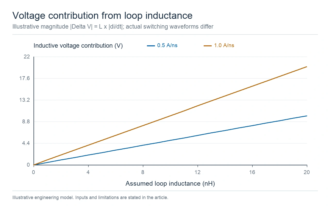
Illustrative voltage contribution at fixed slopes of 0.5 and 1.0 A/ns; actual switching waveforms require evaluation.
The Semikron Danfoss note on DC-link inductance, revision 04, reports switching behavior under a stated module test setup. It shows why inductance, overvoltage, current slope, and switching losses have to be considered together. Its module measurements should not be transferred as numerical limits to a different PCB power stage.
One reported comparison uses 600 V, 600 A, 2 Ω gate resistance, and a 150°C junction condition while varying DC-link inductance from 35 to 85 nH. Under those conditions the note reports a 25% decrease in turn-on energy and a 14% increase in turn-off energy. Those public experimental results show why the direction of one loss term cannot be assumed for another. They are separate from the fixed-slope arithmetic used in our sensitivity table and are not PCB qualification data.
| Assumed loop L | Assumed slope | Calculated |ΔV| | Comparison |
|---|---|---|---|
| 5 nH | 0.5 A/ns | 2.5 V | Lower L and slower slope |
| 5 nH | 1.0 A/ns | 5 V | Only L reduced |
| 10 nH | 0.5 A/ns | 5 V | Only slope reduced |
| 10 nH | 1.0 A/ns | 10 V | Reference example |
Do not equate this contribution with the complete peak voltage at a switch. The bus condition, parasitic capacitance, device behavior, ringing, and measurement reference all affect that peak. Nor does a smaller estimated loop L by itself establish the lowest total switching loss. Use the estimate to select a geometry or switching condition for further evaluation, then check the waveform under the required operating range.
Use loop inductance consistently in that comparison. Adding the isolated partial inductances of nearby outgoing and return conductors without their mutual coupling can misrepresent the complete connection. Identify the extraction ports and the included package or capacitor connections. If one model includes a device package while the other ends at PCB pads, compare them again on the same boundaries before attributing the difference to routing.
The cross-section compares an outgoing conductor and a nearby return at two schematic separations. It explains why both routes must be reviewed together. No absolute inductance or improvement percentage is inferred from the drawing; real extraction must include the actual dimensions and connected structures.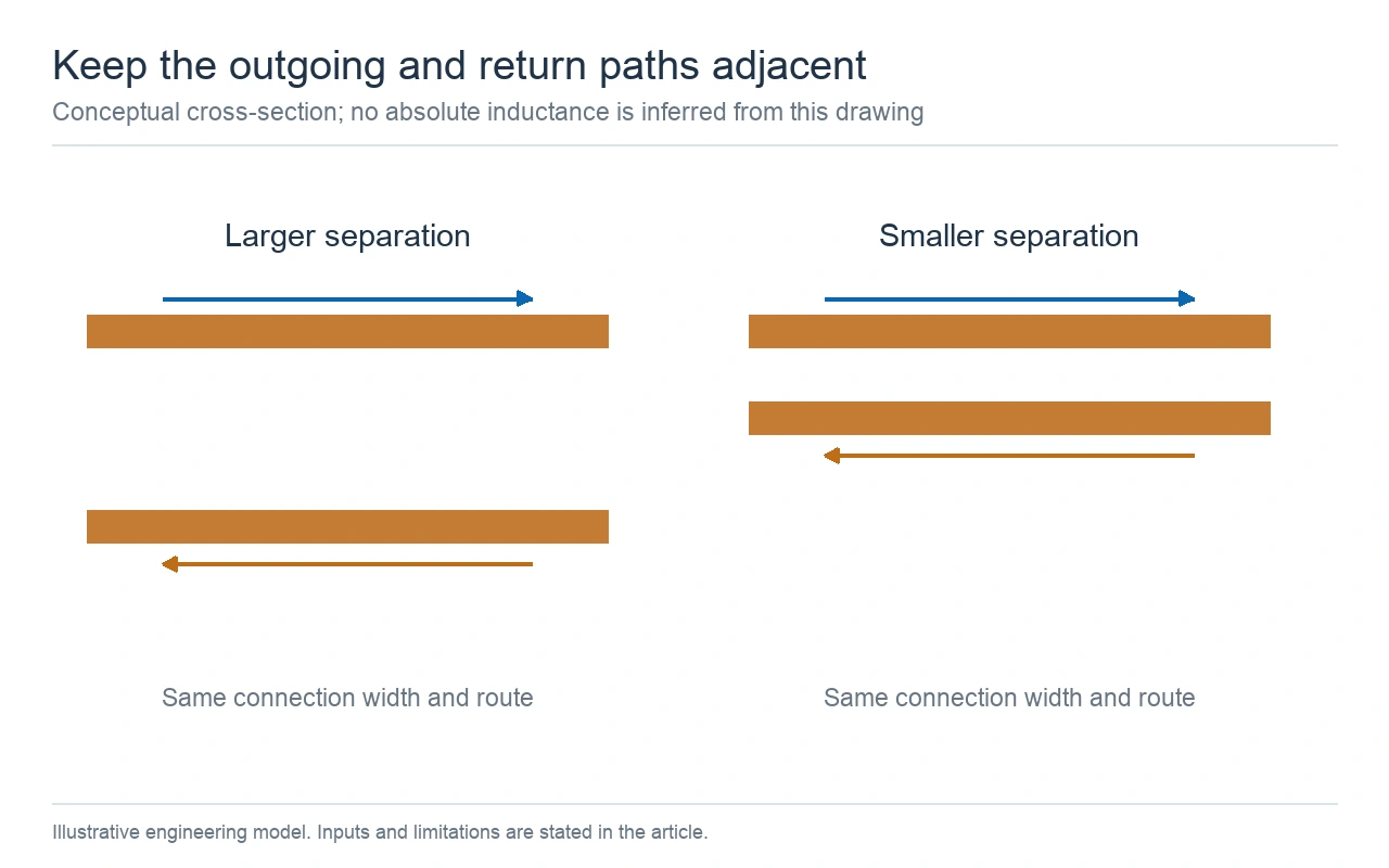
Conceptual connection comparison, not to scale; no absolute inductance or improvement percentage is inferred.
When moving a capacitor to the opposite side of a board, include its vias in the connection model. A short vertical path with adjacent outgoing and return vias can differ from a route that is short on the top view but returns elsewhere. The EPC motor-drive layout discussion illustrates construction choices for its own reference design. It supports evaluating the whole connection rather than applying a same-side placement rule without context.
A local capacitor supplies the difference between the current demanded by the power stage and the current arriving from the source during a chosen interval. Use that deficit waveform in the calculation. Motor phase current is not automatically the capacitor deficit current. Switching state, other active phases, and source response determine the relationship.
ΔQ = ∫ Ideficit(t) dt
Charge-only ΔV = ΔQ / Ceffective
For constant deficit: ΔV = Ideficit × Δt / Ceffective
Assume a 10 A constant deficit lasting 200 ns. The charge requirement is 10 × 200 × 10−9 = 2 μC. With 10 μF of effective capacitance, the charge-only drop is 0.20 V. With 40 μF, it is 0.05 V. Both results use the same imposed current waveform. They do not include the source response or prove that either capacitor arrangement is suitable for an inverter.
The droop plot shows only the charge term for the constant-deficit example. Its straight lines are computed values, not oscilloscope traces. The capacitance labels refer to effective capacitance at the operating condition, rather than the nominal total printed on component packages.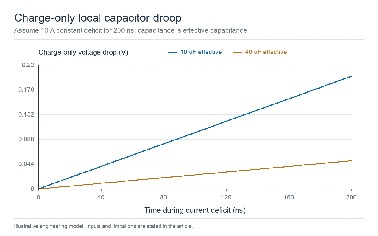
Charge-only calculation with effective capacitance; ESR, ESL and source response are excluded.
Check DC bias, temperature, and tolerance when determining that effective value. Series connection changes it too: two equal capacitors in series have half the capacitance of one, before other operating effects are applied. A change made to meet a voltage requirement must therefore be carried back into the charge calculation. Record the chosen network, not just a sum of nominal component values.
ESR and ESL contribute on different parts of the transient. A hypothetical 10 A current step through 2 mΩ of ESR contributes 0.020 V. An assumed 1 nH series inductance at 1 A/ns contributes 1 V during that slope. These terms help explain why increasing nominal capacitance can leave a fast voltage feature unresolved. Their maxima need not occur at the same time, so do not add unrelated peak numbers and call the sum a predicted waveform.
A device-specific network model and measurements can include damping, package behavior, and the changing source current. Use those tools to evaluate the actual excursion. The simplified calculations are most useful before layout freeze, when an engineer can still adjust the connection or compare a different capacitor network without treating a provisional result as a release criterion.
Separate a fast local voltage feature from a sustained rise in the DC bus during regeneration. A motor can return energy to a bus whose source cannot absorb it. Increasing a nearby bypass capacitor may change a short transient while leaving that longer energy balance unresolved. Define the event duration and the source's ability to receive current before deciding whether the issue belongs to commutation geometry, bulk energy storage, or another system function.
The fabrication review should identify the copper regions, layer spacing, and interconnections that the electrical model assumes. Finished copper and the route's narrowest section affect DC resistance. The dielectric separation between outgoing and return regions affects the field geometry. A manufacturing change can influence one of these without improving the other, so specify which dimensions and connections need engineering approval.
KnownPCB's heavy-copper PCB product page is the starting point for the relevant manufacturing construction. Submit the actual layer and copper combination. A thick-copper capability does not establish a particular loop inductance, switching waveform, or allowable current for every routing shape.
The plating-line photograph illustrates a manufacturing step that contributes to finished copper construction. It does not show a measured copper thickness for this example or verify a motor-drive electrical result. Match inspection evidence to the dimensions called out in the fabrication package.
Pattern plating provides manufacturing context; copper thickness and switching performance require separate evidence.
Keep the motor-drive application requirements with the electrical review. The industrial and automation application page provides the broader project context. The selected circuit, operating environment, isolation requirements, and required validation still need to be defined by the system team. Separate those requirements from the hypothetical examples in this article.
Prepare a release note that identifies the approved stackup, critical connection geometry, assumed parasitic model, and operating condition used for comparison. Name changes that require the design team to rerun the model. For evaluation, specify the voltage measurement endpoints and the current measurement used to obtain di/dt. Probe connection and bandwidth must be appropriate before two layouts' waveforms can be compared.
Use KnownPCB's quality-management framework to discuss the bare-board inspection evidence needed for the order. Electrical connectivity testing is separate from switching-waveform evaluation on an assembled drive. Send the fabrication package and controlled features through the engineering contact page so the manufacturing review addresses the same connections used in the design model.
October/09/2026ENIG Nickel and Gold Thickness: Drawings, XRF, and Reports

September/06/2026High Current PCB Design: Current Paths, Copper, Vias & Thermal Limits
October/10/2026SMPS PCB Layout: Hot Loops, Return Paths, and EMI Checks
October/15/2026Stacked vs. Staggered Microvias: Choose by Constraint
February/25/2026High-Frequency PCB Performance: Low Dk/Df, Controlled Impedance and Low Signal Loss
Proven by 7 industries, 4000+ customer projects
Please contact us at sales@knownpcb.com, ask for engineering support here or use the form below to reach out to KnownPCB | Request a Manufacturing QuoteInclude your quantity, target delivery date and key requirements. File handling and NDA information. |