
112G PAM4 PCB design starts with a defined electrical channel, not a laminate label. The engineer needs the gross serial rate, the signaling format, and the reference planes used by the interface specification. Those choices determine the symbol interval and the frequency at which a loss allowance is evaluated. A board described only as "112G capable" gives purchasing no controlled construction and gives the signal-integrity team no testable channel.
The calculations below separate rate conversion from a hypothetical loss allocation. The first follows from PAM4 arithmetic. The second uses assumed design inputs to explain a planning decision. Neither establishes a KnownPCB acceptance limit or proves that a routed board will pass a particular protocol. Keep that distinction when the numbers move into a stackup request, channel model, or fabrication drawing.
Build the channel budget
PAM4 uses four amplitude levels. Each symbol can represent two gross bits because log2(4) equals 2. If Rb is the gross bit rate in bits per second, the symbol rate Rs is Rb divided by 2. The unit interval used here is one symbol interval, so UI equals 1/Rs. A UI defined from the symbol rate must not be replaced by the shorter reciprocal of the gross bit rate.
Rs = Rb / 2
UI = 1 / Rs
Nyquist frequency = Rs / 2 = Rb / 4
For an illustrative gross rate of 112 Gb/s, Rs is 56 GBd. The symbol interval is 1 divided by 56 billion, or approximately 17.857 ps. The associated Nyquist frequency is 28 GHz. These are rate relationships, not a statement that a PCB needs no useful response above 28 GHz. The selected interface and its channel evaluation define the required frequency coverage.
The level diagram uses normalized amplitude to show the symbol interval. Its transitions are ideal drawing elements, not an eye diagram from a transmitter, receiver, or production PCB. The 17.857 ps label belongs only to the stated 112 Gb/s gross-rate example.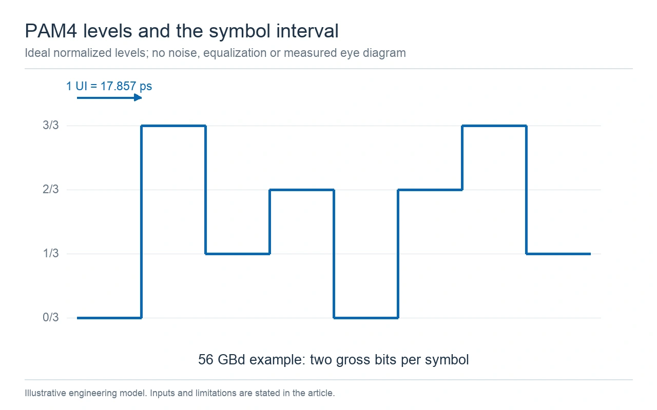
Ideal normalized PAM4 drawing for a 112 Gb/s gross-rate example; this is not a measured eye diagram.
A second example shows why the interface name needs a rate definition. At 106.25 Gb/s gross, PAM4 produces 53.125 GBd, a UI of approximately 18.824 ps, and a Nyquist frequency of 26.5625 GHz. A project using those values must not silently substitute the round-number 112 Gb/s calculations. Record the rate from the actual interface requirements.
The Renesas white paper on 112G PAM4 SerDes jitter discusses the difference between modulation schemes and application-specific clock requirements. Its transmitter and reference-clock limits belong to the interfaces and conditions identified in that document. They are not interchangeable with PCB trace skew or a universal timing allowance.
The paper's interface discussion includes 53.125 GBd, which is the public symbol-rate value used in the second conversion example. The resulting 106.25 Gb/s is its two-bit-per-symbol gross-rate arithmetic. This connection to a published condition does not identify the payload throughput or qualify every design carrying a "112G" label.
The conversion panel keeps both arithmetic examples together. All rates shown are gross rates before any payload-efficiency calculation. If the project specifies a payload rate, first account for the applicable coding, framing, and error-correction overhead before selecting a serial rate.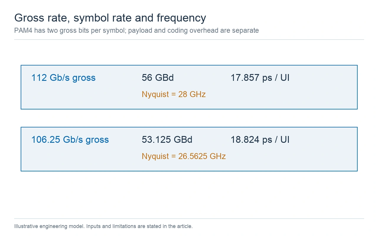
Rate conversions use gross serial rates and two bits per PAM4 symbol; coding and payload efficiency are separate.
A clock frequency is another separate number. A reference clock can be much slower than the baud rate while still influencing transmitter jitter. Specify its frequency, jitter integration band, and applicable receiver or transmitter requirement independently. Multiplying a clock frequency by an arbitrary factor does not establish the lane rate or the permissible PCB mismatch.
A loss result is meaningful only between identified reference planes. A connector-to-connector model, a ball-to-ball model, and a model that includes package interconnects cover different physical paths. Put the endpoints on a drawing. Then list which traces, connectors, launches, and via transitions lie between them. This prevents one team from budgeting a package that another team has already included.
Define the differential quantity being compared. A differential insertion-loss result commonly uses a mixed-mode transmission parameter such as Sdd21. Its magnitude is often reported as a negative number in decibels. A loss allowance is commonly expressed as a positive magnitude. State the sign convention so a reported negative transmission value is not accidentally added as a negative loss contribution.
The channel map separates two PCB sections and a connector between the transmitter and receiver reference planes. It is a bookkeeping diagram. A physical transition that is already part of a connector model must not be allocated again as an independent transition in the same budget.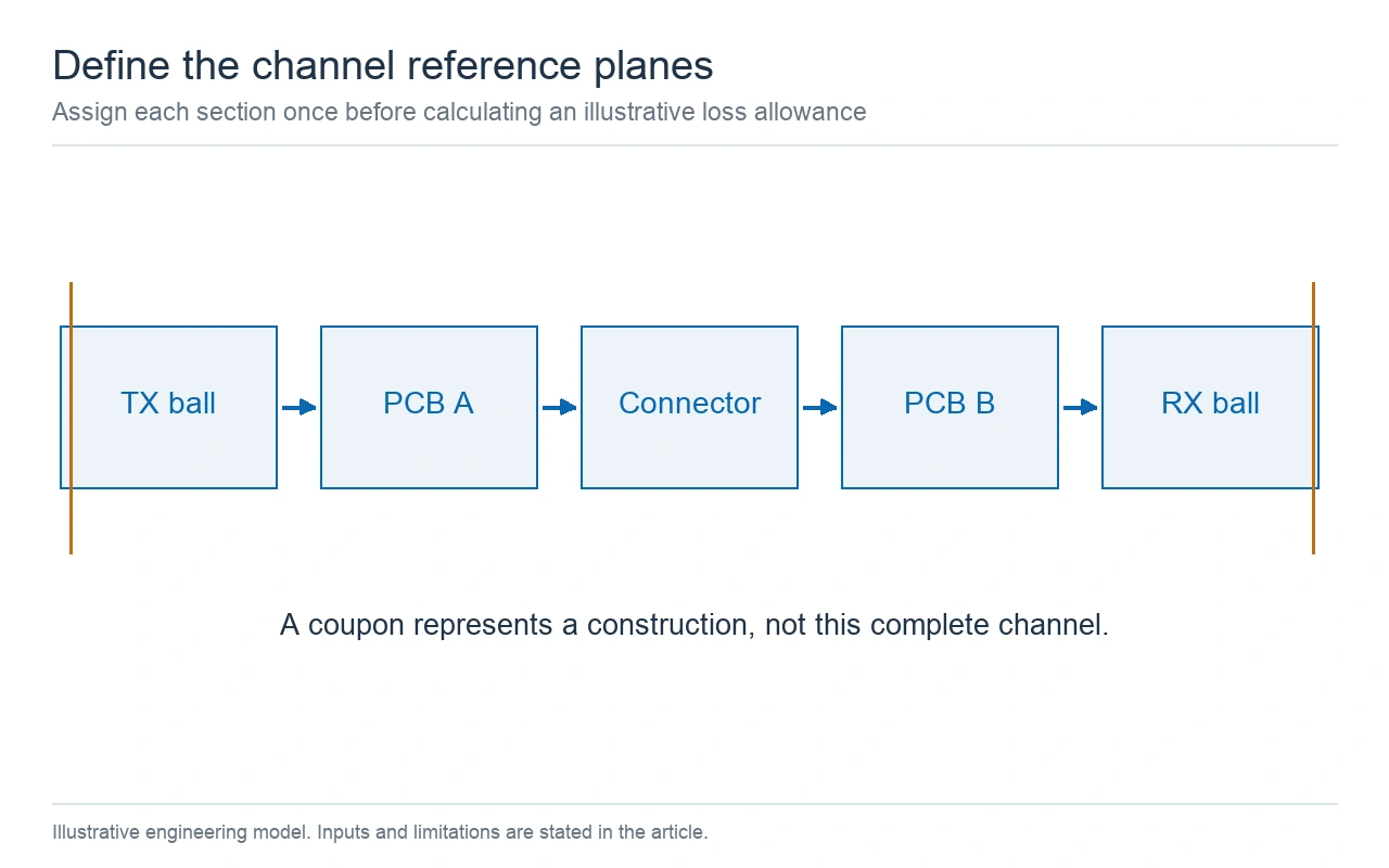
Reference-plane bookkeeping for a hypothetical channel; each physical section is included once.
Frequency-dependent attenuation and the definition of the channel are discussed in AMD XAPP1392's channel insertion-loss section. That application note ties its recommendations to its transceiver context and reference planes. Use the selected device and interface documents to set the project requirement; a value taken from an unrelated long-reach example is not a valid replacement.
Ask for models with compatible port definitions and reference impedances. An uncorrected fixture or launch can change the apparent performance of a test structure. When comparing candidate materials, hold the geometry, copper construction, frequency, and reference-plane definition constant. Otherwise, a favorable material comparison may actually be a different test structure.
For a matched, consistently normalized differential transmission parameter, insertion-loss magnitude in decibels is −20 log10(|Sdd21|). The corresponding transmitted power fraction is 10−IL/10. A hypothetical loss magnitude of 14.2 dB therefore corresponds to a normalized transmission magnitude of about 0.195 and a power fraction of about 0.038. Those quantities answer different questions; neither is the percentage of a receiver's eye opening.
Preserve the differential port pairing and polarity when converting a single-ended model. A four-port connector file and a differential channel model cannot be combined by matching file names alone. Identify the physical ports, their pairing, the reference impedance, and the direction of transmission. Where mode conversion is relevant, retain the needed mixed-mode terms instead of interpreting differential insertion loss as the complete behavior.
Assume an 18 dB planning allowance at 28 GHz. Assume 12 cm of total routed PCB length with an estimated attenuation of 0.8 dB/cm. Allocate 2.0 dB to connectors, 1.6 dB to transitions, and 1.0 dB to other included effects. Every input in this paragraph is hypothetical. The values do not come from a KnownPCB test report or a protocol compliance table.
Trace allocation = length × attenuation per unit length
Total allocated loss = trace allocation + other section allocations
Unused allowance = assumed allowance − total allocated loss
The trace allocation is 12 × 0.8 = 9.6 dB. Adding the other allocations gives 9.6 + 2.0 + 1.6 + 1.0 = 14.2 dB. Subtracting that result from 18 dB leaves 3.8 dB. This is arithmetic for planning sufficiently matched sections. Reflections and interactions between discontinuities require a cascaded channel model; adding isolated loss magnitudes cannot reproduce them.
| Hypothetical scenario at 28 GHz | Trace loss | Total allocation | Unused part of 18 dB |
|---|---|---|---|
| 12 cm at 0.8 dB/cm | 9.6 dB | 14.2 dB | 3.8 dB |
| 12 cm at 1.0 dB/cm | 12.0 dB | 16.6 dB | 1.4 dB |
| 16 cm at 1.0 dB/cm | 16.0 dB | 20.6 dB | −2.6 dB |
The allocation graphic displays the first scenario and its unused allowance. Its bars are calculated from the inputs above, not measured S-parameters. The unused allowance is an arithmetic remainder, not proof of an open eye, a target bit-error rate, or a compliant link.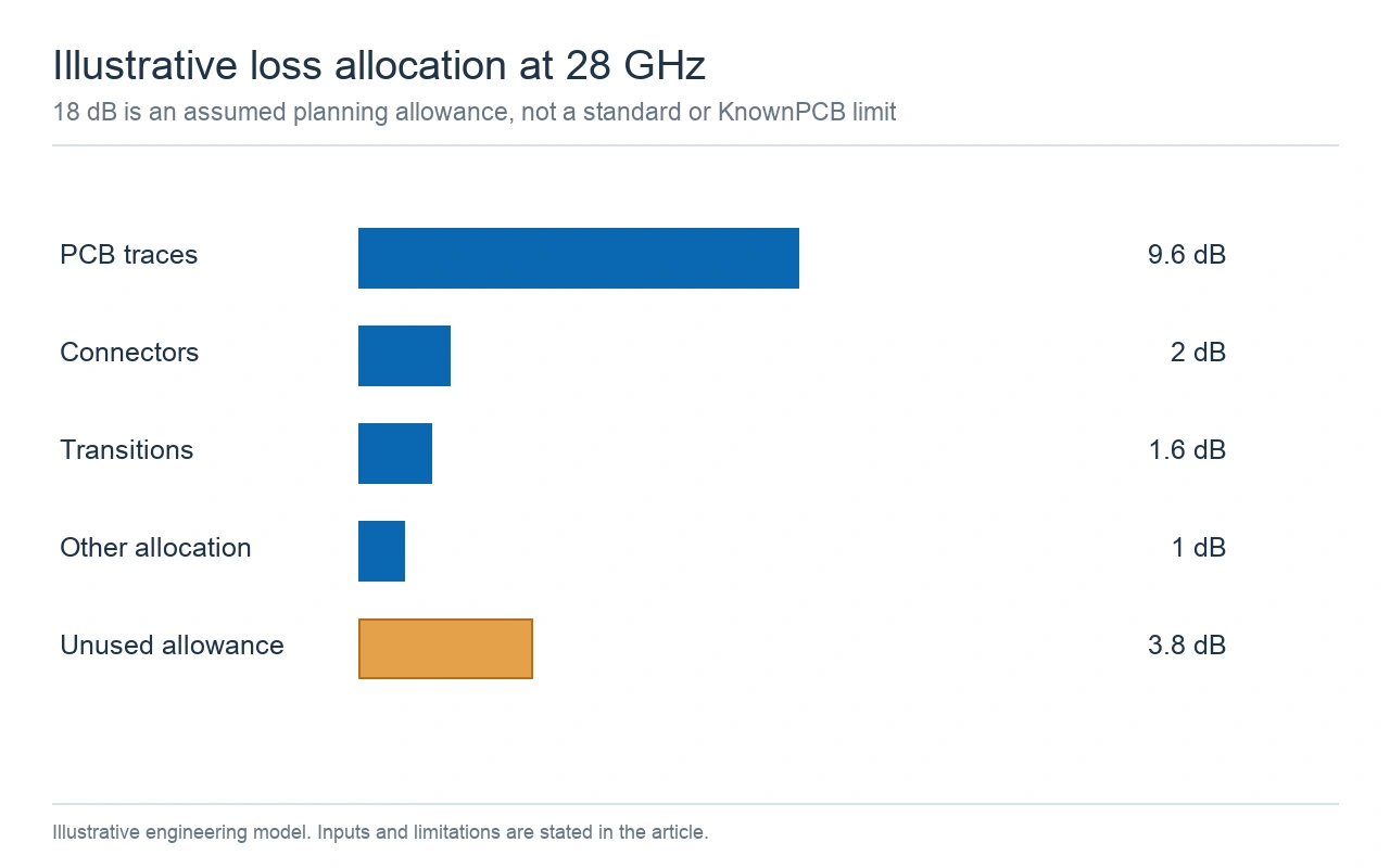
Hypothetical 28 GHz budget: 14.2 dB allocated from an assumed 18 dB allowance, leaving 3.8 dB.
The sensitivity table identifies a useful engineering question. If attenuation changes from 0.8 to 1.0 dB/cm while routing stays at 12 cm, the remainder falls by 2.4 dB. If the route then grows to 16 cm, the assumed allowance is exceeded. That comparison can justify reviewing layer assignment, route length, or a copper option before the board layout is frozen.
Replace each estimate with evidence as the design matures. A material data sheet supplies material properties under stated conditions. A field solver estimates a chosen geometry. A representative test structure measures a fabricated structure. Keep these evidence types labeled in the budget rather than allowing a typical laminate property to become a measured full-channel result.
The 0.8 dB/cm assumption in this example is a value at one frequency. Do not extend it as a frequency-independent line model. A real comparison needs loss versus frequency over the range used by the selected evaluation method. Resonant notches, return loss, and coupling can invalidate a favorable single-frequency total. Retain the frequency grid and the assumptions of each imported model when reviewing a combined result.
Allocate a construction change to the sections it actually affects. Changing a PCB dielectric can alter the routed-line response while leaving a connector's supplied model unchanged. Moving a connector or changing its launch can alter the transition model even if the laminate remains the same. Track those changes separately so a favorable line estimate does not hide an unreviewed launch revision.
The stackup request should identify the routed layers and their reference planes. Include the proposed dielectric system, copper foil option, and finished conductor geometry. Dielectric loss and conductor loss are separate contributors. A lower laminate loss factor does not remove the need to assess copper profile or transitions. Use one controlled construction when comparing model predictions with later samples.
The photographed multilayer PCB illustrates dense routing and connector features that may appear in a high-speed project. Its appearance does not establish a data rate, a material grade, or a measured channel loss. Those statements require the project construction and electrical evidence.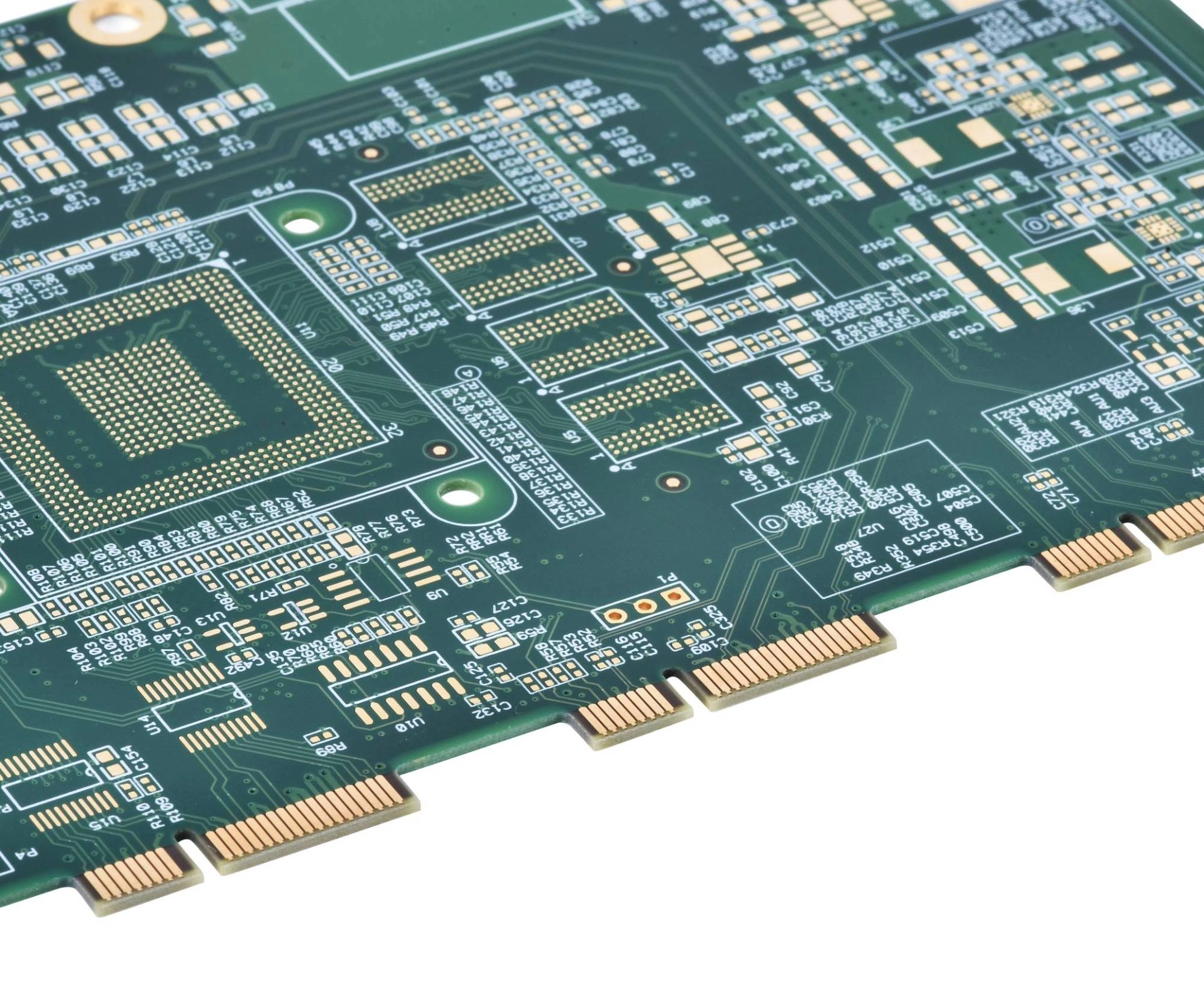
General multilayer PCB context; the photograph does not establish a data rate or measured channel loss.
Review the breakout and each change of reference plane before adding trace length to meet a visual routing pattern. The TI high-speed interface layout guidelines discuss routing symmetry, return paths, and via discontinuities. Apply those principles with the selected interface's requirements. A generic layout guideline does not create a 112G acceptance number.
KnownPCB's RF and high-speed PCB manufacturing page provides the product scope for an engineering discussion. Submit the intended material system and transitions rather than combining unrelated smallest features from different capability rows. The manufacturing response should identify assumptions and any proposed construction changes.
Keep the channel definition with the fabrication revision. Record the gross rate and modulation, the reference planes, the loss frequency, the applicable requirement, and the source of each allocation. Identify which substitutions require a new model or another test. This makes a later material or connector change reviewable without reconstructing the original assumptions from email.
Keep model identity alongside board identity. Record the model file revision, port map, material construction, and any fixture removal used for a measured structure. A later repeat order may use the same routing artwork while a foil option or dielectric thickness has changed. Comparing that lot with an old model is useful only after confirming that the model still represents the released construction.
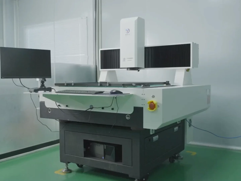
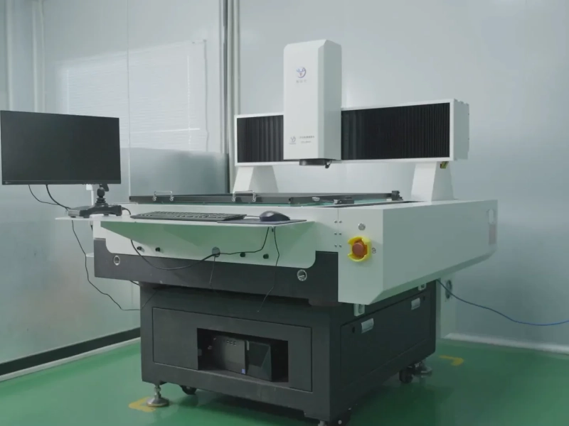
The alignment equipment photograph provides manufacturing context. It does not measure channel insertion loss, jitter, or a 112G eye opening. Use it to illustrate production activity while keeping electrical verification in the model and test records.
Manufacturing alignment equipment is shown as process context, not as electrical channel verification.
A TDR coupon can support impedance control for a representative construction, but its pass result does not establish the full channel's insertion loss. The distinction is developed in KnownPCB's TDR report interpretation article. Request evidence that answers the actual requirement and agree any special measurement or external qualification arrangement before ordering.
Send the channel definition and stackup through KnownPCB's engineering contact page. Include the unresolved entries in the budget and the geometry that cannot change. The resulting review can then address the same electrical path that the design team intends to release.
March/04/2026RFPCB Optimization for Ultrasound Probe Medical Devices
December/06/2025What Are The HDI Board Risks for Radar Modules
October/09/2026ENIG Black Pad: Inspection and Lot Traceability

April/24/2026Aluminum vs Copper vs Stainless Steel MCPCBs: Thermal Performance, Cost and Applications
October/23/2026BMS PCB Design Requirements: Sensing and Fabrication