
On this page
A plated through via can connect a signal on one internal layer while leaving a length of unused barrel below it. That unused length is the residual via stub. It is an open-ended section of transmission line, so its electrical effect depends on length, dielectric environment, via geometry, and the signal edge reaching the discontinuity.
Backdrilling removes much of the unused plated barrel from the opposite board surface after the through hole has been plated. The drill must clear enough barrel to shorten the electrical stub, while stopping before it cuts the target connection or an adjacent layer. A nominal drill depth alone does not tell you the remaining stub unless its reference surface and drill-point geometry are also defined.
The active part of the via runs between the layers that carry the signal. Copper beyond that path is still connected to the via, even though the signal does not use it. In a through-hole board, this unused segment can continue past the signal layer to the board edge. Backdrilling cuts from that edge toward the active layer and leaves a shorter stub.
The drawing below shows the unused plated barrel before drilling and a backdrilled barrel with a short residual section. It only explains the geometry. It does not show a specific layer count, finished hole diameter, drill entry side, or measured result.
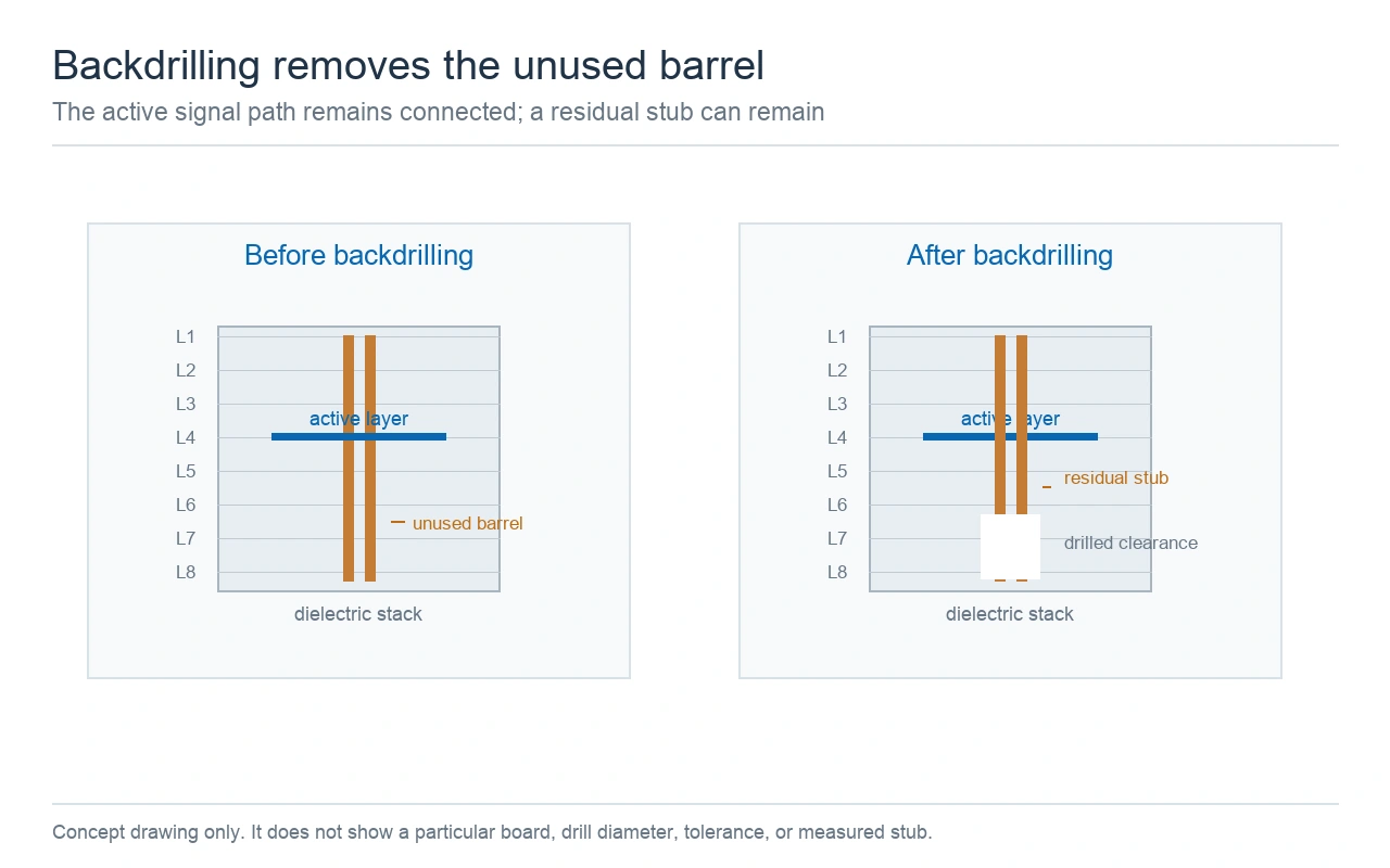
Backdrilling removes an unused section of plated barrel but can leave a residual stub.
KnownPCB already has a separate article on the signal-integrity role of via stubs. This article covers a different task: translating the released layer position and a depth callout into a residual-length estimate, then checking how the stated tolerances move that estimate. The older article describes a single board case; its stackup and process figures are not inputs to the examples below. Read the separate via-stub case discussion.
A backdrill depth can be specified from a board surface, from a target layer, or as an offset from that layer. Those instructions are not equivalent unless they identify the same datum. Ansys HFSS 3D Layout, for example, represents backdrilling by a depth, by a selected layer with an offset, or by a selected layer without an offset. A fabrication drawing needs the same kind of unambiguous choice: which side is drilled, which finished surface anchors depth, and which layer must remain intact. Ansys backdrilling parameter reference.
In the dimension chain here, board thickness H is measured between finished outer surfaces. Target-layer depth z is measured from the top surface to the signal layer. Drill-tip depth Dtip is measured from the finished bottom surface to the deepest point of the tool. Use the same stackup revision for H and z, and use the finished thickness definition that matches the depth program.
A drill point reaches farther into the board than the full-diameter part of the bit. Let q be the axial distance from the deepest tip point back toward the entry surface to the effective barrel-clearance plane. A positive q therefore lengthens the remaining stub relative to a point-only calculation. The size of q depends on tool point geometry, drill diameter, barrel geometry, and the agreed definition of where residual plated copper ends. It must come from the actual tool specification or a measured section, not from a generic constant.
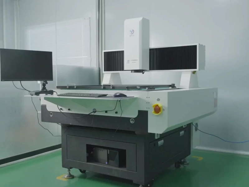
A photo of an X-ray target-drilling station gives manufacturing context. It does not show a backdrill, its depth program, or an inspected residual stub. Use the released drawing and inspection record for those questions.
 A worker at an X-ray target-drilling station, shown as general factory context rather than evidence of backdrill depth.](/upload/image/20261026/xray-target-drilling.webp "[xray-target-drilling.webp](/users/mac/desktop/knownpcb/素材1/weekly-2026-10-26/cn-originals/xray-target-drilling.webp) a worker at an x-ray target-drilling station, shown as general factory context rather than evidence of backdrill depth.")
An X-ray target-drilling station is shown as general factory context; the photograph is not a backdrill measurement.
With those definitions, a point-and-correction estimate is:
Lres = H − z − Dtip + q
This simple geometry estimate does not describe the full drill cone or plated barrel. It assumes the target-layer position and board thickness use the same stackup reference. It also assumes drill depth uses the finished bottom surface and q always means the distance from the deepest point back to the barrel-clearance plane. If the drawing gives depth to the full-diameter cut, do not add q again.
The illustration uses the bottom surface as the drill-depth datum. The blue interval runs from the active layer to the effective barrel-clearance plane. The orange interval q separates that plane from the deepest drill point.
 PCB stack dimension chain showing board thickness H, target-layer depth z, drill-tip depth D_tip, correction q, and residual stub L_res.](/upload/image/20261026/backdrill-layer-depth-chain.webp "[backdrill-layer-depth-chain.webp](/users/mac/desktop/knownpcb/素材1/weekly-2026-10-26/technical/pcb-backdrill-residual-stub/backdrill-layer-depth-chain.webp) pcb stack dimension chain showing board thickness h, target-layer depth z, drill-tip depth d_tip, correction q, and residual stub l_res.")
Measure layer position and drill depth from named surfaces, then account for the drill-point correction.
Example 1: calculate one nominal residual. Let H = 2.40 mm, z = 0.80 mm, Dtip = 1.20 mm, and q = 0.04 mm. The un-drilled barrel below the signal layer would be H − z = 1.60 mm. After drilling, the estimated residual is 2.40 − 0.80 − 1.20 + 0.04 = 0.44 mm. The dimensions are chosen to make the calculation reproducible; they do not describe a KnownPCB job or capability.
Do not replace z with a layer number. "L4" does not say how far the signal layer sits from the reference surface. Use its position in the released stackup, including dielectric thicknesses and construction notes that affect that position. On a mixed-material or sequential-lamination board, the layer order alone may not define a precise enough coordinate for the drill plan.
An open stub can be screened with the first quarter-wave approximation, using propagation speed vp = c / √εeff:
fqw ≈ c / (4 × Lres × √εeff)
Benjamin Dannan's DesignCon 2020 study describes via-stub resonances at roughly a quarter wavelength and explains how drill-depth tolerance can leave a longer stub. The paper also relates stub length to resonance frequency. This supports using the equation as an estimate, not as a measured notch for every stackup. Dannan, "Signal Integrity Characterization of Via Stubs on High-Speed DDR4 Channels," DesignCon 2020.
Continue Example 1 with εeff = 3.8 as an explicit model input. The 1.60 mm unused section before drilling gives an ideal quarter-wave estimate of about 24.0 GHz. The 0.44 mm residual gives about 87.4 GHz. The calculation moves the idealized resonance upward because the remaining line is shorter. It does not prove that a real channel notch lands at either frequency.
The curve below varies residual length and εeff in the same equation. A longer stub lowers the estimated frequency. Increasing εeff also lowers it. Use an effective dielectric constant that matches the field model or measurement. The laminate Dk on a data sheet is not automatically the via's effective value.
 Ideal quarter-wave frequency versus residual via-stub length for assumed effective dielectric constants of 3.2, 3.8, and 4.4.](/upload/image/20261026/via-stub-quarter-wave-frequency.webp "[via-stub-quarter-wave-frequency.webp](/users/mac/desktop/knownpcb/素材1/weekly-2026-10-26/technical/pcb-backdrill-residual-stub/via-stub-quarter-wave-frequency.webp) ideal quarter-wave frequency versus residual via-stub length for assumed effective dielectric constants of 3.2, 3.8, and 4.4.")
The ideal open-stub estimate falls as residual length or effective dielectric constant increases.
Nominal depth gives one answer. A design review needs the range that remains when board thickness, target-layer position, programmed drill depth, and tool correction move within their stated bounds. For independent worst-case limits, calculate both ends explicitly:
Lmin = Hmin − zmax − Dmax + qminLmax = Hmax − zmin − Dmin + qmax
Example 2: combine a hypothetical tolerance stack. Start from Example 1 and assume H = 2.40 ± 0.05 mm, z = 0.80 ± 0.03 mm, Dtip = 1.20 ± 0.05 mm, and q = 0.04 ± 0.02 mm. The minimum is 2.35 − 0.83 − 1.25 + 0.02 = 0.29 mm. The maximum is 2.45 − 0.77 − 1.15 + 0.06 = 0.59 mm. These are deliberately hypothetical bounds to teach the arithmetic, not a factory tolerance or KnownPCB promise.
Using the same assumed εeff of 3.8, the long end of that range gives about 65.2 GHz and the short end gives about 132.6 GHz in the ideal model. The wider spread comes from adding worst-case dimension limits. If the minimum residual approaches zero, check whether the drill could cut the active pad or target layer. Do not report a negative stub. A tolerance calculation needs a measurement basis for every input.
The next table varies one parameter at a time around the 0.44 mm nominal residual. Other inputs stay at Example 1 values. The low frequency in each range corresponds to the longer residual; the high frequency corresponds to the shorter one.
| Parameter varied | Assumed bound | Residual range | Ideal fqw range at εeff = 3.8 |
|---|---|---|---|
| Board thickness H | ±0.05 mm | 0.39 to 0.49 mm | 78.5 to 98.6 GHz |
| Target-layer depth z | ±0.03 mm | 0.41 to 0.47 mm | 81.8 to 93.7 GHz |
| Drill-tip depth Dtip | ±0.05 mm | 0.39 to 0.49 mm | 78.5 to 98.6 GHz |
| Tip correction q | ±0.02 mm | 0.42 to 0.46 mm | 83.6 to 91.6 GHz |
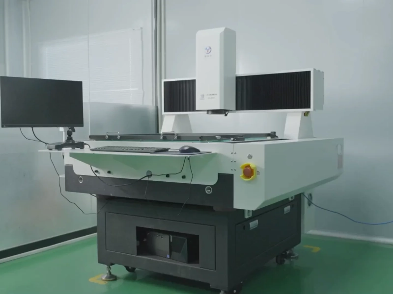
A separate photo of a drilling-equipment line provides broad process context. It does not establish that the visible machines performed the backdrill in a specific build, nor does it document layer registration, depth control, or cross-section results.

The drilling-line photograph is general factory context, not evidence of a backdrill tolerance or inspection result.
The visual range below uses combined worst-case arithmetic for Example 2. Its endpoints come from the stated hypothetical values, not from a production capability record.
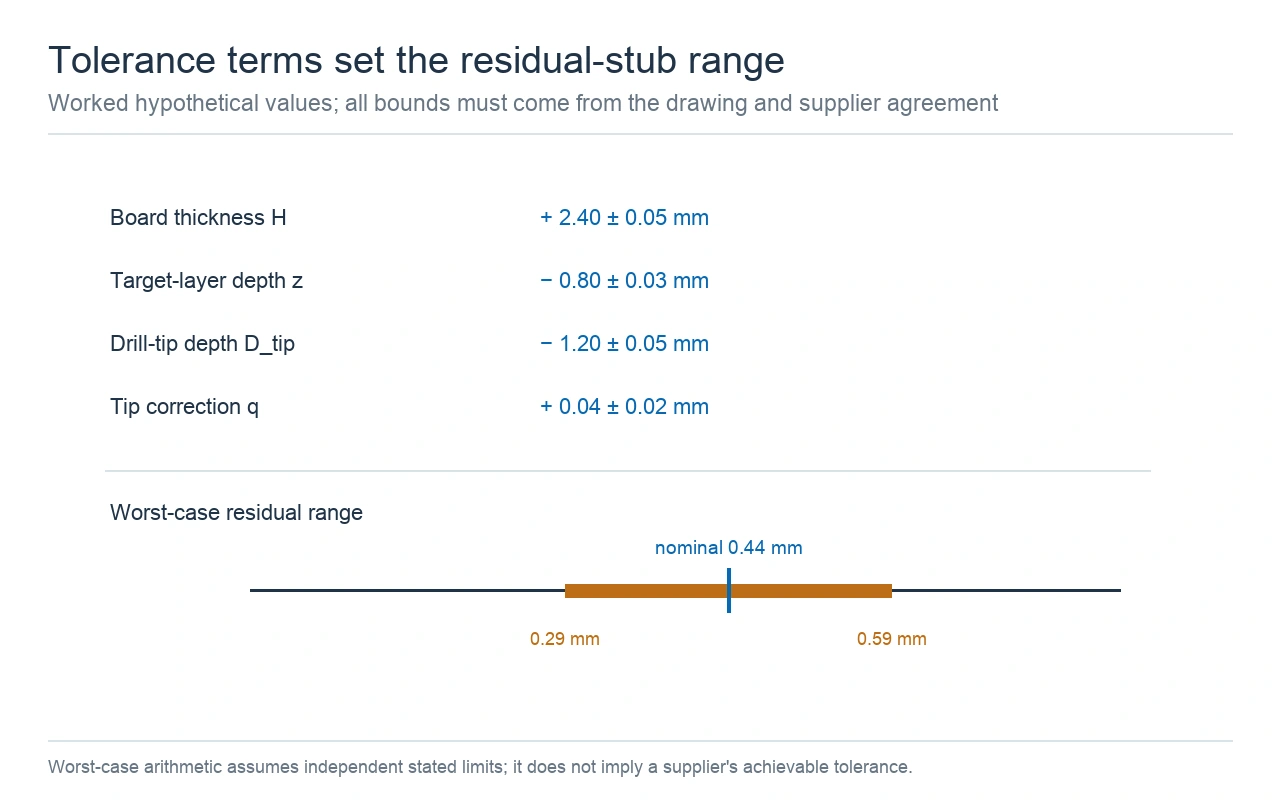
Independent hypothetical limits produce a 0.29 mm to 0.59 mm residual range.
Jianmin Zhang and co-authors studied a model for predicting residual stub length after backdrilling. Their abstract describes measurement comparisons and a sensitivity study of stub length and resonant frequency. That work supports treating the inputs as linked. A depth change alters the remaining stub length and shifts the resonance estimate. It does not set a universal depth tolerance for another shop or stackup. Zhang et al., "Stub Length Prediction for Back-Drilled Vias using a Fast Via Tool".
The quarter-wave equation treats the stub as a uniform open line. A real via includes pads, anti-pads, ground planes, a return path, nearby vias, and a drill-point transition. Those structures add capacitance and coupling, so the measured resonance can differ from the estimate. Ansys modeling, a 3D electromagnetic solver, or a measured S-parameter coupon can represent more of that geometry than the one-dimensional formula.
The first notch does not by itself show that a channel meets its limits. Compare it with the signal spectrum, Nyquist frequency, edge rate, insertion-loss limit, return-loss target, and margin at the receiver. If the calculation puts a resonance near a frequency of concern, update the via model and channel simulation. Do not use the estimate as a pass or fail result.
A cross-section can verify the barrel left at the sampled location. It does not prove the electrical result for every via on the panel. If the acceptance plan uses test coupons, state how the coupon matches the target via area. Also state whether the reported stub is a maximum, an average, or a single-section measurement. Keep the measurement definition aligned with q in the calculation.
A fabrication note should identify the signal layer and drill side, the finished surface datum, the target layer or tip depth, the allowed depth tolerance, the final backdrill diameter, and any layers or pads that must not be cut. State the maximum residual-stub requirement and the verification method. If a tool-point correction is used, define whether the depth number refers to the drill point, the full-diameter cut, or another machine reference.
Ask the fabricator to review the complete stackup and drill drawing before releasing a critical depth. A useful review response names the datum, the controlling thickness, how the tip is calibrated, the remaining clearance to the target layer, and how a sample will be inspected. That exchange makes the design assumption visible before panels are drilled.
KnownPCB's public product capability table lists backdrilling for high speed and low loss boards. It says special constructions are reviewed against the stackup and manufacturing files. The high-frequency and high-speed PCB page is the related service page. Neither page sets a universal residual-stub tolerance. Send the layer sequence, target signal layers, drill side, and electrical limit for a design-for-manufacturing review.
Use the equations here to check the assumptions and estimate the effect of a residual stub. Use the fabrication drawing, agreed process limits, and the project's signal-integrity plan to make the final decision.
March/24/2026HDI Microvia Cracking | Failure Analysis Steps
March/10/2026How 0.2–1.2 mil Solder Mask Thickness Affects 100 Ω Differential Impedance and Insertion Loss

April/24/2026Aluminum vs Copper vs Stainless Steel MCPCBs: Thermal Performance, Cost and Applications
October/06/2026ENEPIG vs ENIG for PCB Pads: Palladium, Inspection and Finish Choice
October/06/2026PCB Plating Voids: Causes, Inspection and Prevention