Blog & Design Guide

PCB differential pair skew is a time difference. A length report can help you find where the difference may come from, but matching two copper lengths does not always make their electrical delays equal. The line layer, local dielectric field, via transitions, package delay, and the interface timing rule all affect the result.
Start with the timing relationship that the design needs to meet. Then convert the allowed time difference into a first-order length estimate for the relevant line type. This keeps a PCB differential pair skew check tied to its actual budget instead of turning it into a blanket routing rule.
In this article
Intra-pair skew is the arrival-time difference between the positive and negative legs of one differential pair. If the P leg and N leg have different delays, the receiver sees an imbalance between the two waveforms. That imbalance can add common-mode energy and can reduce the margin available to the interface.
Inter-pair skew compares the arrival time of one differential pair with another pair in a timing group. A design may need to align several data lanes to a clock or to a shared sampling window. That requirement is separate from matching P to N within each lane. The protocol and device documents define which signals belong in each group and what time limit applies.
Use the same terms throughout the drawing and review. In this article, “intra-pair” means P versus N on one lane. “Inter-pair” means one differential lane versus another lane in a specified group. Some design notes use these labels inconsistently, so include the actual signal names and comparison points in the timing table.
Skew is also different from jitter. Skew describes a relative delay between two paths. Jitter describes how an edge or clock period changes over repeated transitions. A clock specification may include both, but a PCB trace-length conversion only estimates the path-delay part of skew.
Also state the two reference points used for the comparison. A trace length measured from a package ball to a connector is not the same comparison as a board-only route from the component pad to a test point. Keep the package and connector terms either inside the budget or outside it by agreement. Otherwise, two engineers may calculate different “PCB skew” values from the same layout.
The drawing below separates the two comparisons. It is a concept diagram, not a timing result for a board or protocol.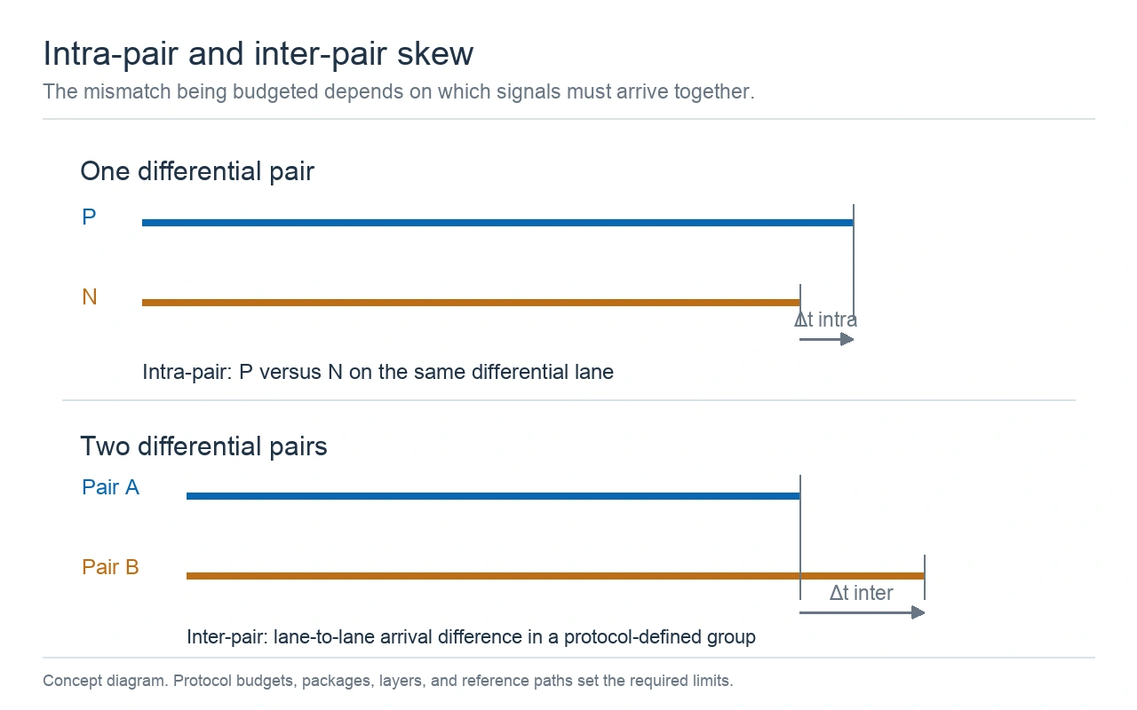
Concept diagram of intra-pair and inter-pair timing comparisons. The drawing does not set a protocol limit.
For a uniform transmission-line segment, a useful first-order estimate is:
Δt = ΔL × √εeff ÷ c
Here, Δt is the time difference in seconds, ΔL is the copper-path length difference in metres, εeff is the effective dielectric constant for that line geometry, and c is the speed of light in vacuum, about 299,792,458 metres per second. If you use millimetres and picoseconds, keep the unit conversion explicit.
The estimate assumes the compared length lies in the same line environment. It is a useful way to check a short mismatch on one layer. It is not a complete model of a route that crosses several layers, different reference planes, connectors, or packages. For those paths, calculate or simulate each segment with its own delay and add the results.
For a simple check, use the absolute length difference between the two paths being compared. Keep the identity of the longer path separately because the sign can matter when you combine the board result with package or connector delay. Do not compare one trace's total routed length with another trace's length only after the via transition. Both paths need the same start and stop points.
Worked example one uses a hypothetical effective dielectric constant of 3.2 and a length mismatch of 5 mm. The estimated delay is 5 mm × √3.2 ÷ 299.792 mm/ns, or about 0.0298 ns. That equals 29.8 ps. The value illustrates the conversion only. It is not a recommended mismatch or a measured board result.
The chart below shows the same first-order conversion for εeff = 3.2. The straight line makes the proportional relationship visible. Use the actual field-solver delay for the stackup and trace shape being reviewed.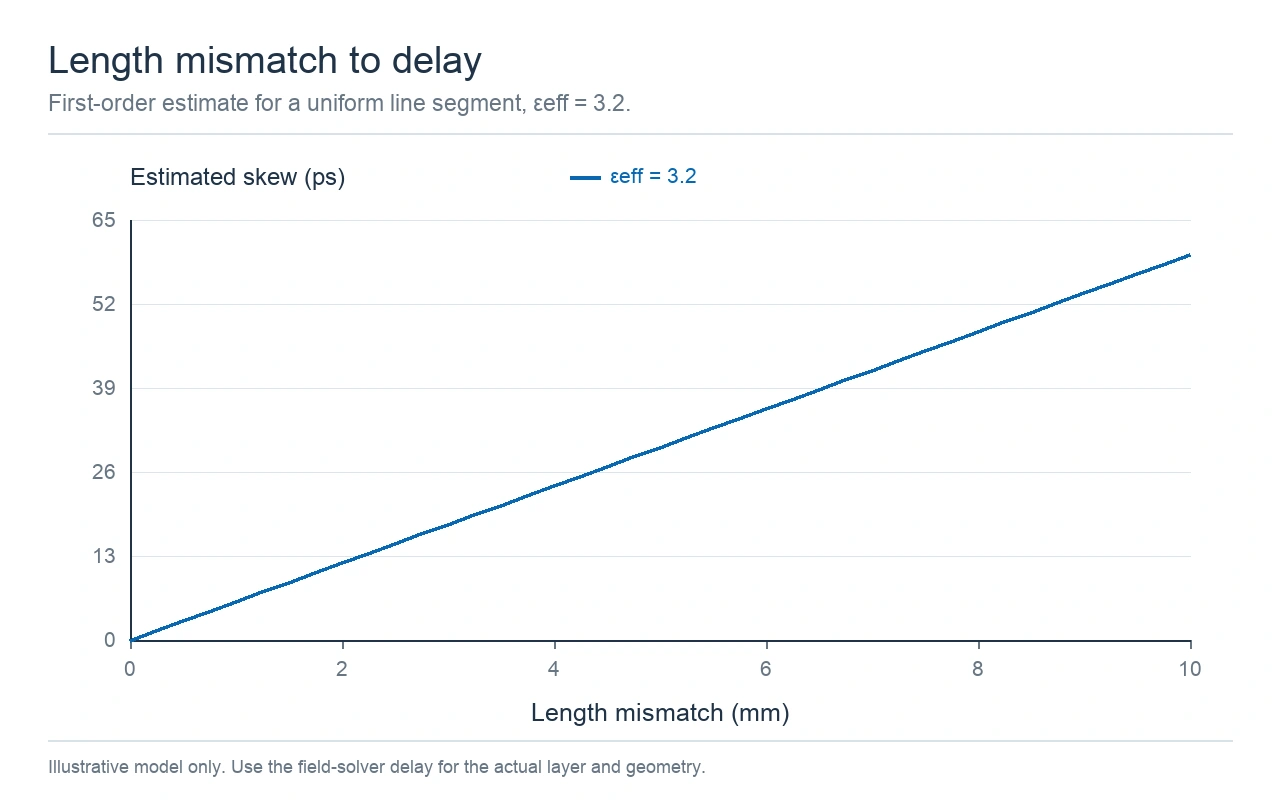
Calculated delay for one uniform line segment at εeff = 3.2. The curve is a model, not a measured trace.
A finished-board photograph can show a high-frequency PCB construction, but it does not reveal the length or delay of a specific differential route. The board image below is included only as product context.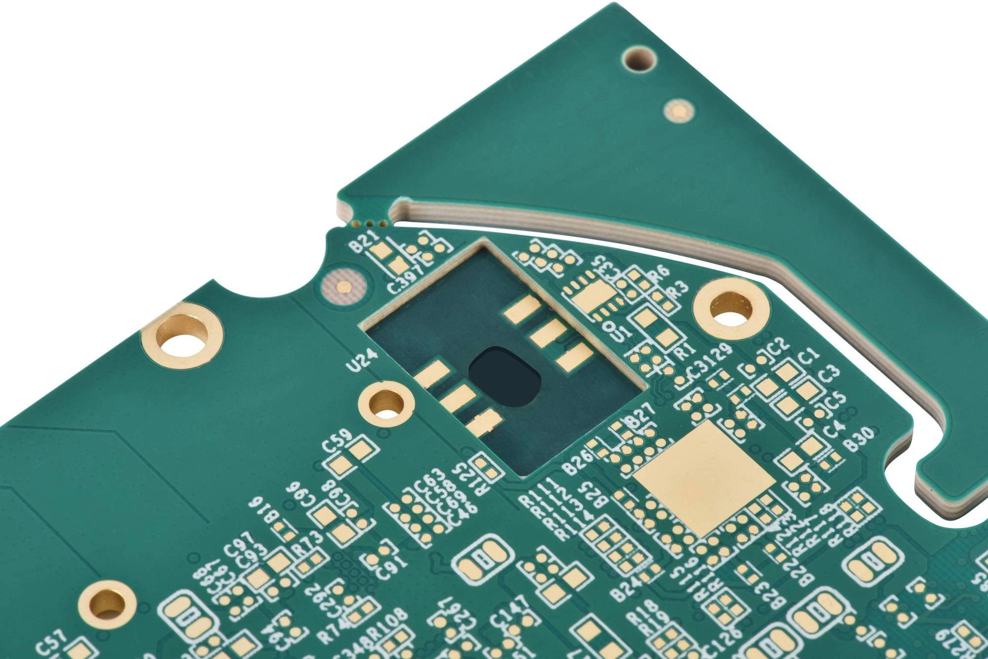
Finished PCB image for visual context only. No trace length or skew measurement is inferred from the photograph.
Design reviews often begin with a time limit and ask how much PCB length difference that limit represents. Rearranging the same estimate gives:
ΔL = c × Δt ÷ √εeff
Worked example two uses a 10 ps budget and εeff = 3.2. The first-order length equivalent is 299,792,458 m/s × 10 ps ÷ √3.2, or about 1.68 mm. That equals about 66 mil. This is an estimate for a uniform line section. It does not mean a design with 66 mil of mismatch automatically passes its interface requirement.
If 10 ps is the end-to-end budget for a link, first reserve the portion used by the package, connector, cable, or other channel elements. The remaining board allowance may be smaller. If the specification already gives a PCB-only limit, do not subtract those elements again. The budget definition decides which case applies.
The effective dielectric constant changes the conversion. The table keeps the time budget fixed at 10 ps and shows how the equivalent length changes for three illustrative εeff values. These values are sensitivity inputs, not laminate datasheet limits or a claim about one KnownPCB stackup.
| Illustrative εeff | Delay per 1 mm | Length for 10 ps |
|---|---|---|
| 2.8 | 5.582 ps | 1.792 mm |
| 3.2 | 5.967 ps | 1.676 mm |
| 3.8 | 6.502 ps | 1.538 mm |
As εeff rises, the line delay per millimetre rises, so a fixed time allowance corresponds to less copper length. The figure compares the same relationship across the three inputs. It does not define an acceptable protocol skew value.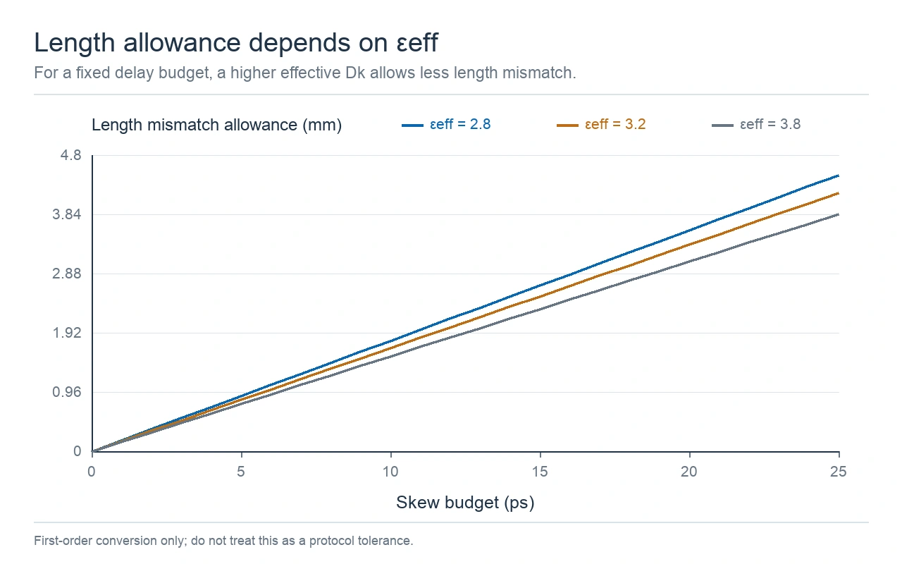
Length allowance for a first-order uniform-line estimate. The effective dielectric constants are illustrative.
εeff is a field-weighted value for the transmission line. It depends on the trace width, spacing, dielectric thickness, nearby reference planes, solder mask, and the amount of the field that extends outside the dielectric. A microstrip and a stripline can have different propagation delays even when they use the same laminate family.
The bulk Dk on a material datasheet describes a material test condition. It is not automatically the εeff needed by the length-to-delay formula. A field solver or a validated line model should use the actual layer dimensions and dielectric construction. If your route changes from microstrip to stripline, calculate those sections separately.
Fiber weave adds local variation. Woven glass and epoxy do not have the same dielectric properties. If the P leg passes through a different mix of glass and resin than the N leg, their local propagation velocities can differ even if the CAD lengths match. TI describes this fiber-weave effect and several ways designers try to reduce the difference in its High-Speed Interface Layout Guidelines.
A PCB panel photograph shows copper artwork and panel edges, but it does not show the glass-weave path under a particular routed pair. The image below is a manufacturing view only. It cannot confirm the dielectric seen by either leg.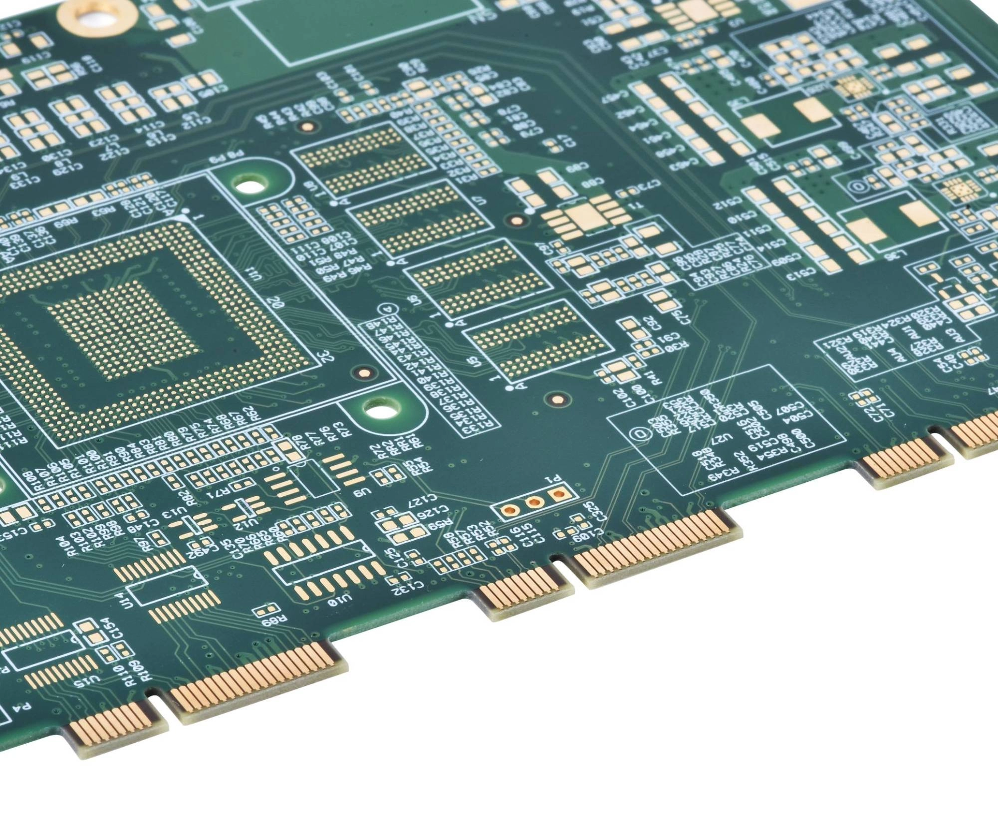
PCB panel photograph for manufacturing context. It does not show internal glass weave or a measured delay.
A via changes the signal environment. The barrel, pads, anti-pads, reference-plane openings, and return vias affect the transition. If the P and N transitions are not electrically alike, the difference may remain even when the visible copper lengths match. A route that moves between layers also uses more than one εeff.
AMD's XAPP1392 discusses intra-pair skew from glass weave and via transitions. It recommends placing a correction on the same layer where the skew occurs, before the signal enters a via, and checking the tuning structure in the actual channel. That recommendation does not replace the interface budget or a channel simulation. Read the specific AMD intra-pair skew guidance before applying it to a design.
Do not treat a serpentine as a delay adjustment with no electrical cost. Closely spaced parallel sections can couple to one another, change the local impedance, and add discontinuities. The correction should be as short and local as the design allows, then checked against the differential impedance and channel response. The diagram below shows one possible location for local tuning. Its shapes are not dimensions for your board.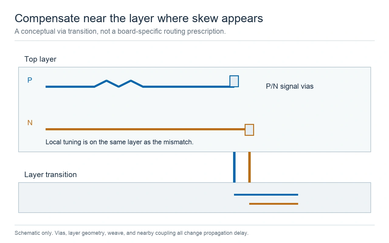
Concept sketch of local timing correction before a layer transition. It does not show a validated routing solution.
A via stub is a different issue from P-to-N skew. A long unused barrel section can create a frequency-dependent impedance discontinuity. Matching P and N path delay does not remove that resonance. TI's high-speed layout report treats via stubs as a signal-integrity issue, while AMD's XAPP1392 discusses where to place a skew correction. Keep the checks separate in the review.
KnownPCB's articles on return-path stability in an HDI stackup and via stubs in high-speed PCB channels discuss related layer and via effects. They cover different signal-integrity questions from the length-to-delay conversion in this article.
Start with the device or protocol requirement and name the signals it compares. Record whether the limit applies to P versus N, one lane versus another, or a wider clock and data group. Do not copy a length tolerance from a different interface or device. TI's High-Speed Layout Guidelines for Signal Conditioners and USB Hubs gives routing examples for the devices and interfaces in that report. It is a useful reference for those parts, not a universal skew budget.
Next, separate the PCB allowance from the rest of the channel. Package traces, connectors, cables, vias, and device-side timing can use part of the total budget. If the interface specification gives an end-to-end limit, the PCB should not consume the entire allowance by default.
For the PCB route, record the layer, line type, stackup revision, effective dielectric value or solver output, and the length difference being compared. If the route crosses layer types or vias, calculate each region with its own delay. Keep the assumed values beside the result so another engineer can repeat the estimate.
A useful review record can fit in one row per timing group. Include the signal names, the start and stop references, the specified skew type, the total time limit, the package allowance, the board estimate, the assumed εeff values, and the method used to check the result. This record makes a later stackup or package change easier to review because the original assumptions remain visible.
Use the formula as a screening calculation. Confirm the final route with the method required by the design, such as a field solver or an agreed channel analysis. A first-order length conversion can show whether a budget is plausible. It cannot prove that a differential link meets timing, impedance, or signal-integrity requirements.
Proven by 7 industries, 4000+ customer projects
Please contact us at sales@knownpcb.com, ask for engineering support here or use the form below to reach out to KnownPCB | Request a Manufacturing QuoteInclude your quantity, target delivery date and key requirements. File handling and NDA information. |